
The Center for Climatic Research focuses on interdisciplinary research regarding the Earth’s climate system, including the causes and impacts of historical, ongoing, and projected climate variability and change, with geographic focuses that span from local to global scale. The center’s diverse activities and societal contributions include the training of students and postdoctoral researchers as the next generation of climate scientists, development of guidance for state government and regional stakeholders regarding climate change impacts and adaptation, and advancement of scientific understanding of the coupled Earth system.
Tools for Tracking Climate Change
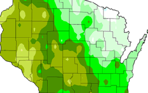
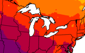
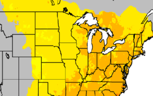
CCR scientists have developed easy-to-understand maps that show historical information and climate projections in Wisconsin and Midwest. The maps provide insights into how temperature, precipitation, length of growing season, and other variables might change in the future.
Excellence in Climate Science
CCR scientists have strong expertise in the areas of climate modeling and climate dynamics, climate impacts, past climates, carbon cycling, terrestrial and aquatic ecosystems, and feedbacks between the atmosphere and earth’s surface.
CCR has a distinguished tradition of over 50 years of excellence in climate science. Its past directors include fellows of the American Geophysical Union and members of the National Academy of Sciences, while its alumni are found in leading atmospheric and geoscience departments around the country. CCR faculty and scientists are at the leading edge of their disciplines.

News and Events
Latest News
- Wisconsin Rural Partnerships Institute brings international climate science program to hundreds of rural studentson March 24, 2025
- Meet the 2025 Distinguished Teaching Award winnerson March 18, 2025
- Excellence in outreach recognized with Bassam Z. Shakhashiri Public Science Engagement Awardon March 10, 2025
- Chance of Atlantic Ocean Circulation Collapse Difficult to Assess, Study Showson February 12, 2025
- Preparing Wisconsin’s rural communities for extreme weather eventson January 2, 2025
Support CCR
The Center for Climatic Research advances understanding of the climate system through interdisciplinary investigations of past, present, and future climates and the application of this knowledge for societally relevant purposes. Gifts to CCR play a crucial role in enhancing the breadth and quality of our research and educational programs.